Preppin' Data 2020: Week 6 challenge solution
Here is my solution for Peppin’ Data 2020, Week 6. This challenge was about conversion rates: identifying the best and the worst exchange rates for each week as well as the weekly variance of sales values.
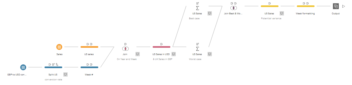
My solution in Tableau Prep
Original challenge and data set on Preppin’ Data’s blog.
Step 1: Sales table: calculating the US sales
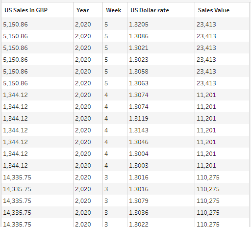
Let’s look at the original sales table for this challenge. All sales are recorded in British Pounds, however, we can infer the amount of the US sales as the split between sales in the UK and US is shown as a percent of total sales.
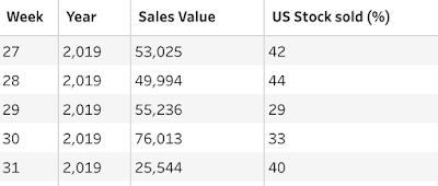
Original sales table where all sales are in GBP
To find the absolute amount of the US sales, we need to add the Cleaning step and create the following calculation called US Sales in GBP:
ROUND([Sales Value]*([US Stock sold (%)]/100), 2)The ROUND function in this calculation rounds the number for the US sales to two decimal places.
Before moving to next step, I removed the US Stock sold (%) field as we won’t need it further.
Step 2: Conversion rates table: extracting the US Dollar rate
Now let’s look at the conversion rates table in the image below. To use the rate in our calculations, we need to extract the actual rate from the British Pound to US Dollar field.
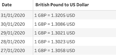
Original exchange rates table
Let’s start with adding the Cleaning step and updating the British Pound to US Dollar field so it’s just a number. To avoid creating duplicated fields, let’s write the following calculated field that I called British Pound to US Dollar (same as the current field) so the calculation’s result replaces the original British Pound to US Dollar field:
TRIM( SPLIT( [British Pound to US Dollar], " = ", 2 ) )In this calculation, we say that our delimiter is ' = ', and we want to go from the beginning of the string and extract the second group of characters after the appearance of our delimiter (that’s why we use '2' in the calculation). This will keep only the exchange rate in the British Pound to US Dollar field now. We can rename this field as US Dollar rate for clarity.
This field still needs some cleaning, so let’s click on the three dots icon in the US Dollar rate field’s header, and select Clean > Remove Letters. To complete, we need to change the data type of this field to Number (decimal).
Step 3: Conversion rates table: finding the week’s number
As we need to identify the best and the worst exchange rates on a weekly basis, we need to roll up our daily exchange rates to a weekly level. We can do it by using a DATEPART function. This function returns a part of a given date as an integer, for example, the week number.
Let’s add a new Cleaning step and create a calculated field called Week:
DATEPART('week', [Date])Now we need to extract the year for each week as this table has rates for both 2019 and 2020. The calculation for our new Year field should look as follows:
YEAR([Date])Step 4: Joining sales and conversion rate tables
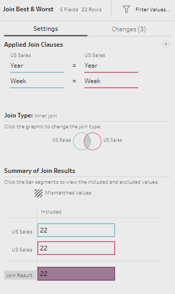
Before we can identify the max and the min sales values, we need to match the rates to the actual sales figures, i.e. join our sales and rates tables. Let’s add the Join step, and choose the Year and Week fields as join clauses.
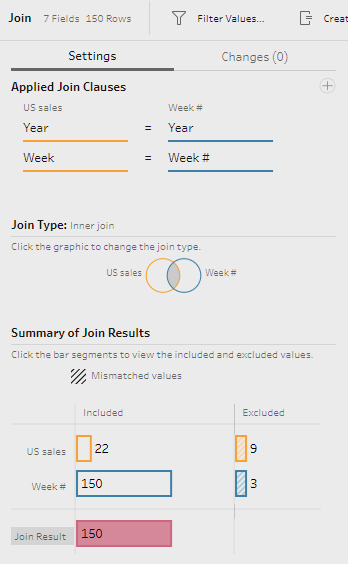
Join step settings
Now we have a table with multiple rows for each week with exchange rates at a certain date during this week.
Remember to remove the duplicated fields Week-1 and Year-1 before moving to the next step.
Step 5: Calculating the UK sales in GBP and converting the US sales into US Dollars
Let’s add the Cleaning step after the join. Now we need to convert the amount of the US sales into US dollars by creating a new calculated field called US Sales in USD:
ROUND([US Sales in GBP]*[US Dollar rate],2)Next step is to calculate the amount of the UK sales in GBP by creating a new calculated field called UK Sales in GBP:
[Sales Value]-[US Sales in GBP]Step 6: Finding the max and min sales value for the US in USD
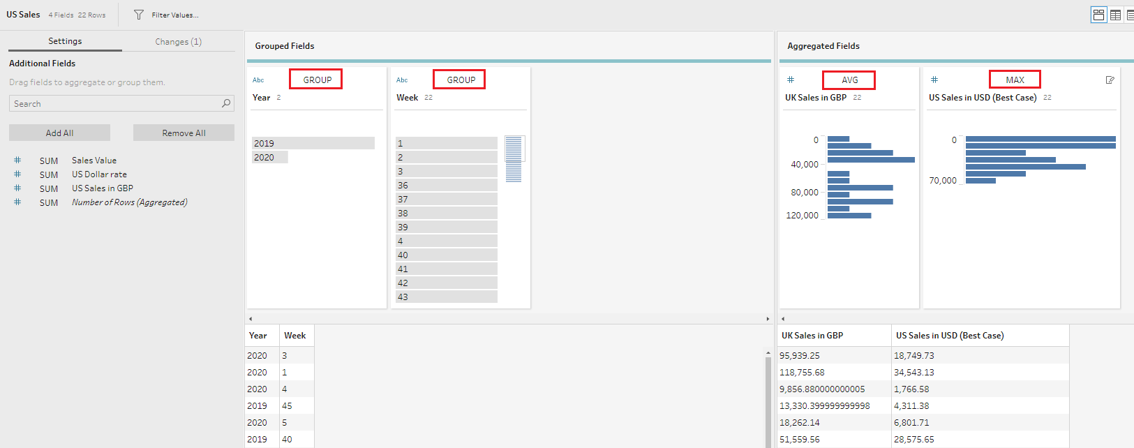
Now that we have all our sales values calculated, we need to identify the max and the min sales values based on different exchange rates for a particular week. For this we need to bring two separate Aggregate steps and configure them as follows:
For max sales volume
Group by Year and Week fields, and aggregate UK Sales in GBP (using AVG aggregation to bring only one number back) and UK Sales in USD fields (using MAX aggregation to bring the highest amount back)
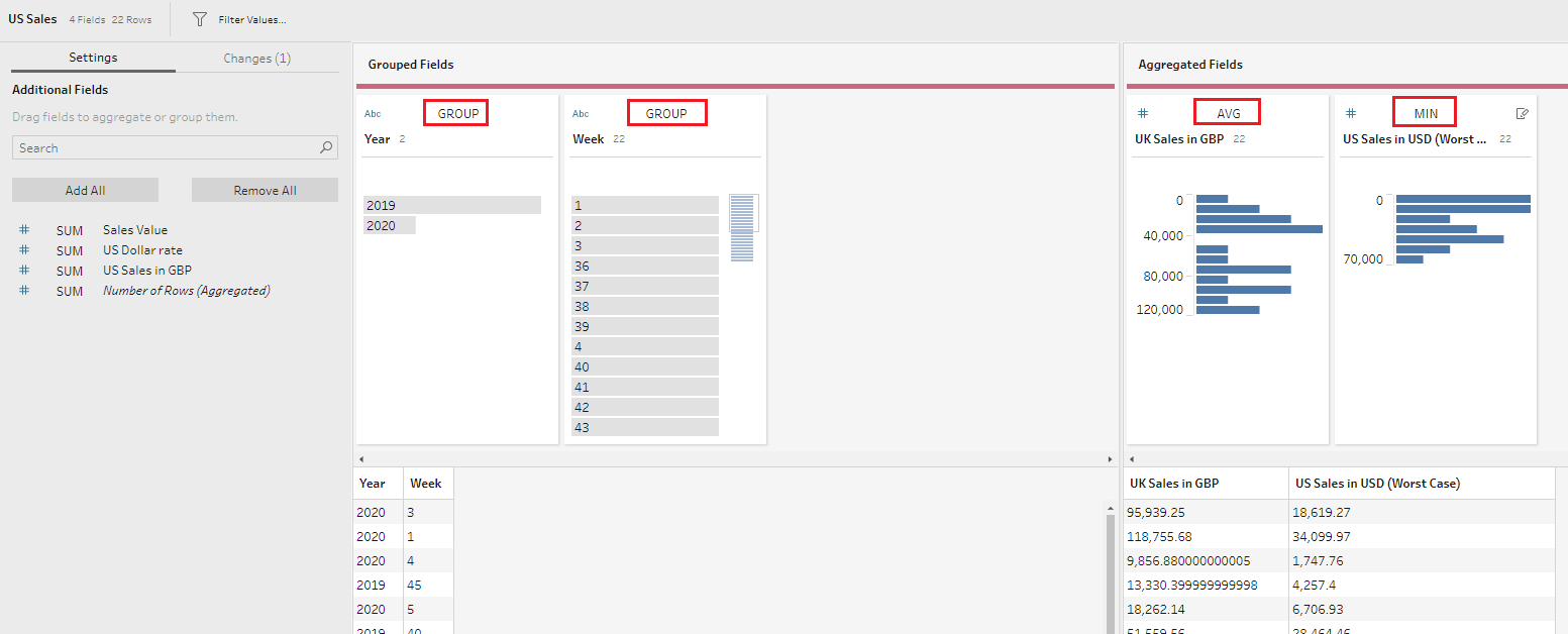
For min sales volume
Group by Year and Week fields, and aggregate UK Sales in GBP (using AVG aggregation to bring only one number back) and UK Sales in USD fields (using MIN aggregation to bring the lowest amount back)
Step 7: Creating a combined table
To calculate the variance between the max and min sales values we need to add the Join step and combine the outputs of both Aggregate steps, selecting the Year and Week fields as join clauses.
Here we should remove the duplicated Week-1 and Year-1 fields. I also rounded up the UK Sales in GBP field with the following calculated field:
ROUND([UK Sales in GBP], 2)Step 8: Calculating the variance in sales values
There are just two things left to complete in the challenge: calculate the variance sales and format the week.
Let’s start with the variance and add the Cleaning step with a simple calculated field called US Sales potential variance:
ROUND([US Sales in USD (Best Case)]-[US Sales in USD (Worst Case)], 2)Step 9: Formatting the Week field
The final output for this challenge requires a particular format for the Week field: for example, for the first week of 2020 it should read as ‘wk 1 2020’.
To get this format, let’s add a new Cleaning step and create a calculated field to update the existing Week field:
'wk ' + STR([Week]) + ' ' + STR([Year])The STR function here changes the data type of the Week and Year fields into a string, allowing us to concatenate them together in the needed format.
Now we should remove the Year field, and our final output is ready:
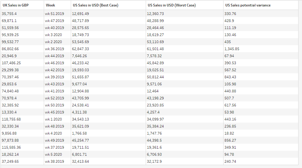
And here is the completed flow for this challenge which you can download from my GitHub repository:
Let me know if you have any questions.